Patient Event Sequencing – Output Generation

Using the tabular output generated by pes_process, this function will build a graph to visualize the results. Each function configuration will output a bespoke ggplot. Theming can be adjusted by the user after the graph has been output using + theme(). Most graphs can also be made interactive using make_interactive_squba()

Usage

pes_output(process_output, large_n = FALSE, large_n_sites = NULL)

Arguments

process_output

tabular input || required

The tabular output produced by pes_process

Note any patient-level results generated are not intended to be used with this function.

large_n

boolean || defaults to FALSE

For Multi-Site analyses, a boolean indicating whether the large N visualization, intended for a high volume of sites, should be used. This visualization will produce high level summaries across all sites, with an option to add specific site comparators via the large_n_sites parameter.

large_n_sites

vector || defaults to NULL

When large_n = TRUE, a vector of site names that can add site-level information to the plot for comparison across the high level summary information.

Value

This function will produce a graph to visualize the results from pes_process based on the parameters provided. The default output is typically a static ggplot or gt object, but interactive elements can be activated by passing the plot through make_interactive_squba. For a more detailed description of output specific to each check type, see the PEDSpace metadata repository

Examples

#' Source setup file
source(system.file('setup.R', package = 'patienteventsequencing'))

#' Create in-memory RSQLite database using data in extdata directory
conn <- mk_testdb_omop()

#' Establish connection to database and generate internal configurations
initialize_dq_session(session_name = 'pes_process_test',
                      working_directory = my_directory,
                      db_conn = conn,
                      is_json = FALSE,
                      file_subdirectory = my_file_folder,
                      cdm_schema = NA)
#> Connected to: :memory:@NA

#' Build mock study cohort
cohort <- cdm_tbl('person') %>% dplyr::distinct(person_id) %>%
  dplyr::mutate(start_date = as.Date(-5000), # RSQLite does not store date objects,
                                      # hence the numerics
                end_date = as.Date(15000),
                site = ifelse(person_id %in% c(1:6), 'synth1', 'synth2'))

#' Build function input table
pes_events <- tidyr::tibble(event = c('a', 'b'),
                            event_label = c('hypertension', 'inpatient/ED visit'),
                            domain_tbl = c('condition_occurrence', 'visit_occurrence'),
                            concept_field = c('condition_concept_id', 'visit_concept_id'),
                            date_field = c('condition_start_date', 'visit_start_date'),
                            vocabulary_field = c(NA, NA),
                            codeset_name = c('dx_hypertension', 'visit_edip'),
                            filter_logic = c(NA, NA))

#' Execute `pes_process` function
#' This example will use the single site, exploratory, cross sectional
#' configuration
pes_process_example <- pes_process(cohort = cohort,
                                   multi_or_single_site = 'single',
                                   anomaly_or_exploratory = 'exploratory',
                                   time = FALSE,
                                   omop_or_pcornet = 'omop',
                                   user_cutoff = 10000,
                                   n_event_a = 1,
                                   n_event_b = 2,
                                   pes_event_file = pes_events) %>%
  suppressMessages()
#> ┌ Output Function Details ──────────────────────────────────────┐
#> │ You can optionally use this dataframe in the accompanying     │
#> │ `pes_output` function. Here are the parameters you will need: │
#> │                                                               │
#> │ Always Required: process_output                               │
#> │                                                               │
#> │ See ?pes_output for more details.                             │
#> └───────────────────────────────────────────────────────────────┘

pes_process_example
#> # A tibble: 3 × 9
#>   site     num_days user_cutoff event_a_name event_b_name       pt_ct total_pts
#>   <chr>       <dbl>       <dbl> <chr>        <chr>              <int>     <int>
#> 1 combined     5628       10000 hypertension inpatient/ED visit     1        12
#> 2 combined     7637       10000 hypertension inpatient/ED visit     1        12
#> 3 combined    10800       10000 hypertension inpatient/ED visit     1        12
#> # ℹ 2 more variables: pts_without_both <int>, output_function <chr>

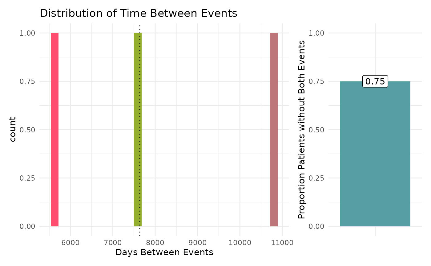
#' Execute `pes_output` function
pes_output_example <- pes_output(process_output = pes_process_example)

pes_output_example[[1]]
#> `stat_bin()` using `bins = 30`. Pick better value `binwidth`.

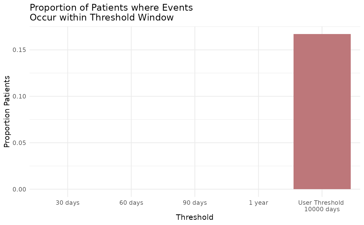
pes_output_example[[2]]


#' Easily convert the graph into an interactive ggiraph or plotly object with
#' `make_interactive_squba()`

make_interactive_squba(pes_output_example[[2]])