Using BOTH tabular outputs generated by cnc_sp_process, this function will build a graph to
visualize the results. Each function configuration will output a bespoke ggplot. Theming can
be adjusted by the user after the graph has been output using + theme(). Most graphs can
also be made interactive using make_interactive_squba()
Usage
cnc_sp_output(
  cnc_sp_process_output,
  cnc_sp_process_names,
  facet_vars = NULL,
  top_n = 15,
  n_mad = 3L,
  specialty_filter = NULL,
  p_value = 0.9,
  large_n = FALSE,
  large_n_sites = NULL
)
Arguments
- cnc_sp_process_output
tabular input || required
The tabular output (with visit-based counts per specialty) produced by
cnc_sp_process- cnc_sp_process_names
tabular input || required
The tabular output (with specialty names & any specialty_name grouping categories) produced by
cnc_sp_processTo see an example of what this file should look like, see
?clinicalevents.specialties::cnc_sp_specialty_names- facet_vars
string or vector || defaults to
NULLA string or vector representing the variables by which the plot should be facet. Accepted values are
clusterand/orvisit_type- top_n
integer || defaults to
15An integer value indicating the cutoff for the top N of each group to display per check
- n_mad
integer || defaults to
3An integer indicating the number of MAD from the median that should be considered the threshold for an anomalous value
- specialty_filter
string or vector || defaults to
NULLAn optional parameter indicating the specialty or specialties to limit to in the analysis
- p_value
numeric || defaults to
0.9The p value to be used as a threshold in the Multi-Site, Anomaly Detection, Cross-Sectional analysis
- large_n
boolean || defaults to
FALSEFor Multi-Site analyses, a boolean indicating whether the large N visualization, intended for a high volume of sites, should be used. This visualization will produce high level summaries across all sites, with an option to add specific site comparators via the
large_n_sitesparameter.- large_n_sites
vector || defaults to
NULLWhen
large_n = TRUE, a vector of site names that can add site-level information to the plot for comparison across the high level summary information.
Value
This function will produce a graph to visualize the results
from cnc_sp_process based on the parameters provided. The default
output is typically a static ggplot or gt object, but interactive
elements can be activated by passing the plot through make_interactive_squba.
For a more detailed description of output specific to each check type,
see the PEDSpace metadata repository
Examples
#' Source setup file
source(system.file('setup.R', package = 'clinicalevents.specialties'))
#' Create in-memory RSQLite database using data in extdata directory
conn <- mk_testdb_omop()
#' Establish connection to database and generate internal configurations
initialize_dq_session(session_name = 'cnc_sp_process_test',
working_directory = my_directory,
db_conn = conn,
is_json = FALSE,
file_subdirectory = my_file_folder,
cdm_schema = NA)
#> Connected to: :memory:@NA
## Turn off SQL trace for this example
config('db_trace', FALSE)
#' Build mock study cohort
cohort <- cdm_tbl('person') %>% dplyr::distinct(person_id) %>%
dplyr::mutate(start_date = as.Date(-5000),
#RSQLite does not store date objects,
#hence the numerics
end_date = as.Date(15000),
site = ifelse(person_id %in% c(1:6), 'synth1', 'synth2'))
#' Prepare input tables
cnc_sp_visit_tbl <- dplyr::tibble(visit_concept_id = c(9201,9202,9203),
visit_type = c('inpatient', 'outpatient', 'emergency'))
cnc_sp_concept_tbl <- dplyr::tibble(domain = 'Hypertension',
domain_tbl = 'condition_occurrence',
concept_field = 'condition_concept_id',
date_field = 'condition_start_date',
vocabulary_field = NA,
codeset_name = 'dx_hypertension')
#' Execute `cnc_sp_process` function
#' This example will use the single site, exploratory, cross sectional
#' configuration
cnc_sp_process_example <- cnc_sp_process(cohort = cohort,
omop_or_pcornet = 'omop',
multi_or_single_site = 'single',
anomaly_or_exploratory = 'exploratory',
codeset_tbl = cnc_sp_concept_tbl,
visit_type_tbl = cnc_sp_visit_tbl,
time = FALSE) %>%
suppressMessages()
#> ┌ Output Function Details ─────────────────────────────────────────┐
#> │ You can optionally use this dataframe in the accompanying │
#> │ `cnc_sp_output` function. Here are the parameters you will need: │
#> │ │
#> │ Always Required: cnc_sp_process_output, cnc_sp_process_names │
#> │ Required for Check: top_n │
#> │ Optional: facet_vars, specialty_filter │
#> │ │
#> │ See ?cnc_sp_output for more details. │
#> └──────────────────────────────────────────────────────────────────┘
cnc_sp_process_example$cnc_sp_process_output
#> # A tibble: 1 × 7
#> specialty_concept_id cluster visit_type codeset_name num_visits site
#> <dbl> <chr> <chr> <chr> <int> <chr>
#> 1 38004446 Essential hyper… outpatient dx_hyperten… 5 comb…
#> # ℹ 1 more variable: output_function <chr>
cnc_sp_process_example$cnc_sp_process_names
#> # A tibble: 1 × 2
#> specialty_concept_id specialty_concept_name
#> <dbl> <chr>
#> 1 38004446 No vocabulary table input
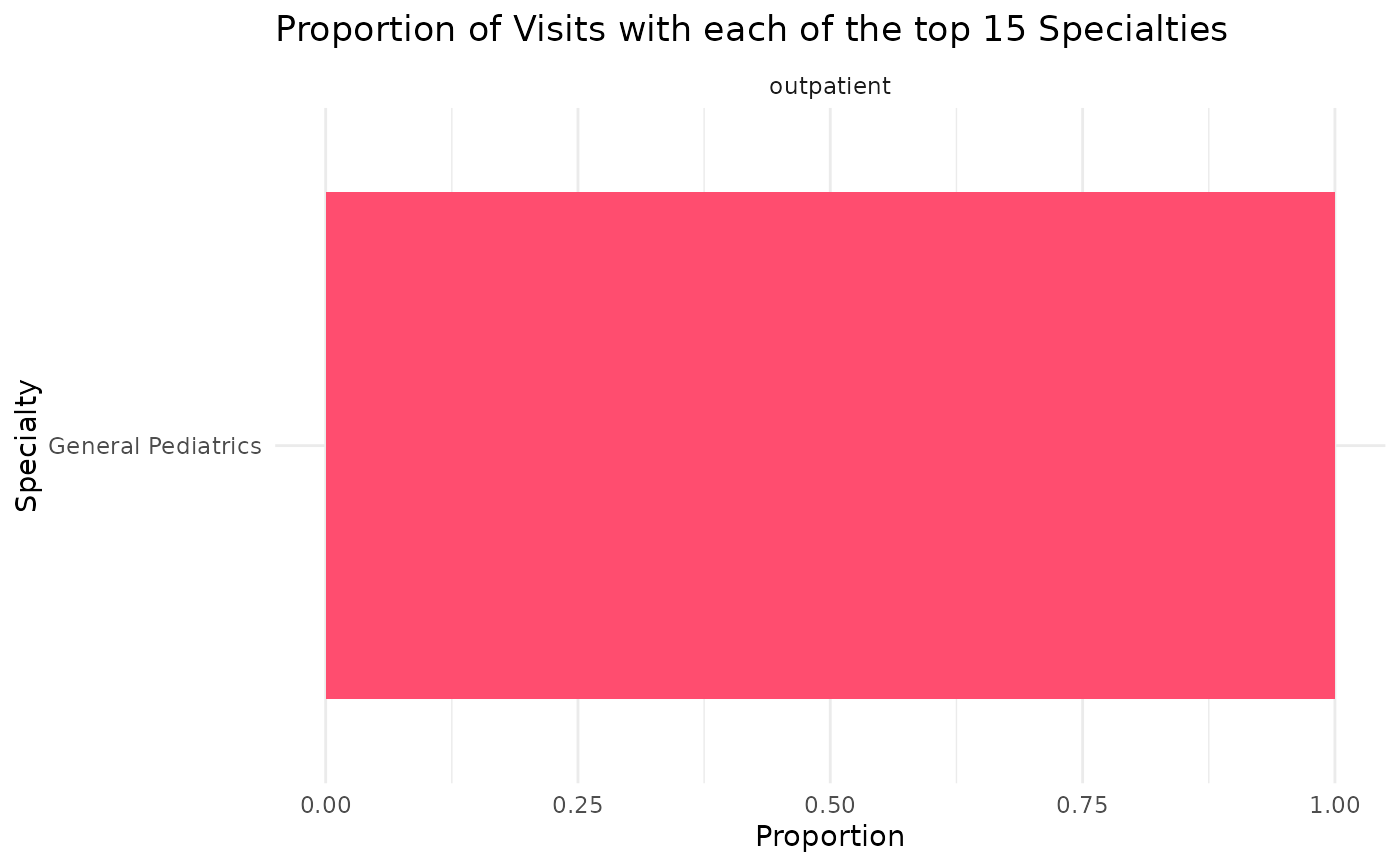
#' Execute `cnc_sp_output` function
cnc_sp_output_example <-
cnc_sp_output(cnc_sp_process_output =
cnc_sp_process_example$cnc_sp_process_output,
cnc_sp_process_names =
cnc_sp_process_example$cnc_sp_process_names %>%
dplyr::mutate(specialty_name = 'General Pediatrics'),
facet_vars = c('visit_type')) %>%
suppressMessages()
cnc_sp_output_example
 #' Easily convert the graph into an interactive ggiraph or plotly object with
#' `make_interactive_squba()`
make_interactive_squba(cnc_sp_output_example)
#' Easily convert the graph into an interactive ggiraph or plotly object with
#' `make_interactive_squba()`
make_interactive_squba(cnc_sp_output_example)