Using the tabular output generated by ca_process, this function will build a graph to
visualize the results. Each function configuration will output a bespoke ggplot. Theming can
be adjusted by the user after the graph has been output using + theme(). Most graphs can
also be made interactive using make_interactive_squba()
Usage
ca_output(
  process_output,
  log_scale = FALSE,
  var_col = "num_pts",
  large_n = FALSE,
  large_n_sites = NULL
)
Arguments
- process_output
tabular input || required
The tabular output produced by
ca_process- log_scale
boolean || default to
FALSEA boolean indicating whether a log transformation should be applied to the y-axis of the output
- var_col
string || defaults to
num_ptsThe name of the column that should be displayed on the plot for Exploratory analyses. The options are:
num_pts: raw patient countprop_retained_start: proportion patients retained from the starting step, as indicated bystart_step_numprop_retained_prior: proportion patients retained from prior stepprop_diff_prior: proportion difference between each step and the prior step
- large_n
boolean || defaults to
FALSEFor Multi-Site analyses, a boolean indicating whether the large N visualization, intended for a high volume of sites, should be used. This visualization will produce high level summaries across all sites, with an option to add specific site comparators via the
large_n_sitesparameter.- large_n_sites
vector || defaults to
NULLWhen
large_n = TRUE, a vector of site names that can add site-level information to the plot for comparison across the high level summary information.
Value
This function will produce a graph to visualize the results
from ca_process based on the parameters provided. The default
output is typically a static ggplot or gt object, but interactive
elements can be activated by passing the plot through make_interactive_squba.
For a more detailed description of output specific to each check type,
see the PEDSpace metadata repository
Examples
#' Build mock study attrition
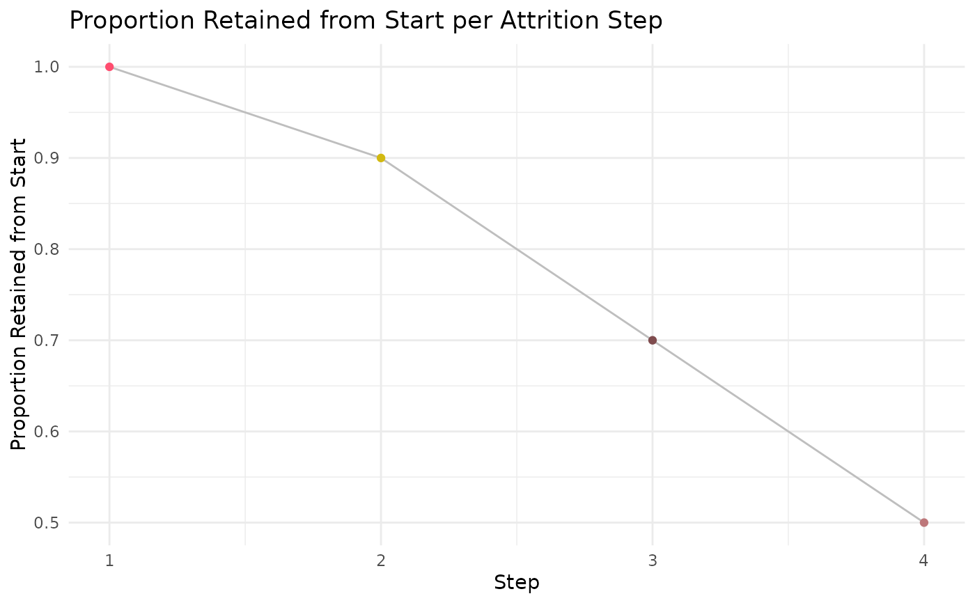
sample_attrition <- dplyr::tibble('site' = c('Site A', 'Site A', 'Site A', 'Site A'),
'step_number' = c(1,2,3,4),
'attrition_step' = c('step 1', 'step 2', 'step 3', 'step 4'),
'num_pts' = c(100, 90, 70, 50))
#' Execute `ca_process` function
#' This example will use the single site, exploratory, cross sectional
#' configuration
ca_process_example <- ca_process(attrition_tbl = sample_attrition,
multi_or_single_site = 'single',
anomaly_or_exploratory = 'exploratory',
start_step_num = 1) %>%
suppressMessages()
#> ┌ Output Function Details ─────────────────────────────────────┐
#> │ You can optionally use this dataframe in the accompanying │
#> │ `ca_output` function. Here are the parameters you will need: │
#> │ │
#> │ Always Required: process_output, var_col │
#> │ Optional: log_scale │
#> │ │
#> │ See ?ca_output for more details. │
#> └──────────────────────────────────────────────────────────────┘
ca_process_example
#> # A tibble: 4 × 9
#> site step_number attrition_step num_pts prop_retained_prior ct_diff_prior
#> <chr> <dbl> <chr> <dbl> <dbl> <dbl>
#> 1 Site A 1 step 1 100 NA NA
#> 2 Site A 2 step 2 90 0.9 10
#> 3 Site A 3 step 3 70 0.778 20
#> 4 Site A 4 step 4 50 0.714 20
#> # ℹ 3 more variables: prop_diff_prior <dbl>, prop_retained_start <dbl>,
#> # output_function <chr>
#' Execute `ca_output` function
ca_output_example <- ca_output(process_output = ca_process_example,
log_scale = FALSE,
var_col = 'prop_retained_start')
ca_output_example[[1]]
 ca_output_example[[2]]
Attrition Step Reference
Step Number
Description
#' Easily convert the graph into an interactive ggiraph or plotly object with
#' `make_interactive_squba()`
make_interactive_squba(ca_output_example[[1]])