Using the tabular output generated by pf_process, this function will build a graph to
visualize the results. Each function configuration will output a bespoke ggplot. Theming can
be adjusted by the user after the graph has been output using + theme(). Most graphs can
also be made interactive using make_interactive_squba()
Usage
pf_output(
  process_output,
  output = NULL,
  date_breaks_str = "1 year",
  domain_filter = NULL,
  visit_filter = NULL,
  large_n = FALSE,
  large_n_sites = NULL
)
Arguments
- process_output
tabular input || required
The tabular output produced by
pf_processNote any patient-level results generated are not intended to be used with this function.
- output
string || defaults to
NULLThe name of the numerical variable from
process_outputthat should be used to generate the plot. This input is required for the following checks:Single Site, Exploratory, Cross-SectionalMulti-Site, Exploratory, Cross-SectionalSingle Site, Anomaly Detection, Cross-SectionalSingle Site, Exploratory LongitudinalMulti Site Exploratory Longitudinal
- date_breaks_str
string || defaults to
1 yearA string that controls the time period division on the x-axis ('1 year', '3 months', etc). This parameter is only required for the
Single Site, Exploratory, Longitudinalcheck.- domain_filter
string || defaults to
NULLA string indicating the domain of interest for plotting. This parameter is required for the following checks:
Single Site, Anomaly Detection, LongitudinalMulti-Site, Anomaly Detection, Longitudinal
- visit_filter
string || defaults to
NULLA string indicating the visit type of interest for plotting. This parameter is required for the following checks:
Multi-Site, Anomaly Detection, Cross-SectionalSingle Site, Anomaly Detection, LongitudinalMulti-Site, Anomaly Detection, Longitudinal
- large_n
boolean || defaults to
FALSEFor Multi-Site analyses, a boolean indicating whether the large N visualization, intended for a high volume of sites, should be used. This visualization will produce high level summaries across all sites, with an option to add specific site comparators via the
large_n_sitesparameter.- large_n_sites
vector || defaults to
NULLWhen
large_n = TRUE, a vector of site names that can add site-level information to the plot for comparison across the high level summary information.
Value
This function will produce a graph to visualize the results
from pf_process based on the parameters provided. The default
output is typically a static ggplot or gt object, but interactive
elements can be activated by passing the plot through make_interactive_squba.
For a more detailed description of output specific to each check type,
see the PEDSpace metadata repository
Examples
#' Source setup file
source(system.file('setup.R', package = 'patientfacts'))
#' Create in-memory RSQLite database using data in extdata directory
conn <- mk_testdb_omop()
#' Establish connection to database and generate internal configurations
initialize_dq_session(session_name = 'pf_process_test',
working_directory = my_directory,
db_conn = conn,
is_json = FALSE,
file_subdirectory = my_file_folder,
cdm_schema = NA)
#> Connected to: :memory:@NA
## turn of SQL trace for example
config('db_trace', FALSE)
#' Build mock study cohort
cohort <- cdm_tbl('person') %>% dplyr::distinct(person_id) %>%
dplyr::mutate(start_date = as.Date(-5000), # RSQLite does not store date objects,
# hence the numerics
end_date = as.Date(15000),
site = ifelse(person_id %in% c(1:6), 'synth1', 'synth2'))
#' Execute `pf_process` function
#' This example will use the single site, exploratory, cross sectional
#' configuration
pf_process_example <- pf_process(cohort = cohort,
study_name = 'example_study',
multi_or_single_site = 'single',
anomaly_or_exploratory = 'exploratory',
visit_type_table =
patientfacts::pf_visit_file_omop,
omop_or_pcornet = 'omop',
visit_types = c('all'),
domain_tbl = patientfacts::pf_domain_file %>%
dplyr::filter(domain == 'diagnoses')) %>%
suppressMessages()
#> ┌ Output Function Details ─────────────────────────────────────┐
#> │ You can optionally use this dataframe in the accompanying │
#> │ `pf_output` function. Here are the parameters you will need: │
#> │ │
#> │ Always Required: process_output │
#> │ Required for Check: output │
#> │ │
#> │ See ?pf_output for more details. │
#> └──────────────────────────────────────────────────────────────┘
pf_process_example
#> # A tibble: 1 × 11
#> study site visit_type domain median_all_with0s median_all_without0s n_tot
#> <chr> <chr> <chr> <chr> <dbl> <dbl> <dbl>
#> 1 example_… comb… all diagn… 0 0 12
#> # ℹ 4 more variables: n_w_fact <dbl>, median_site_with0s <dbl>,
#> # median_site_without0s <dbl>, output_function <chr>
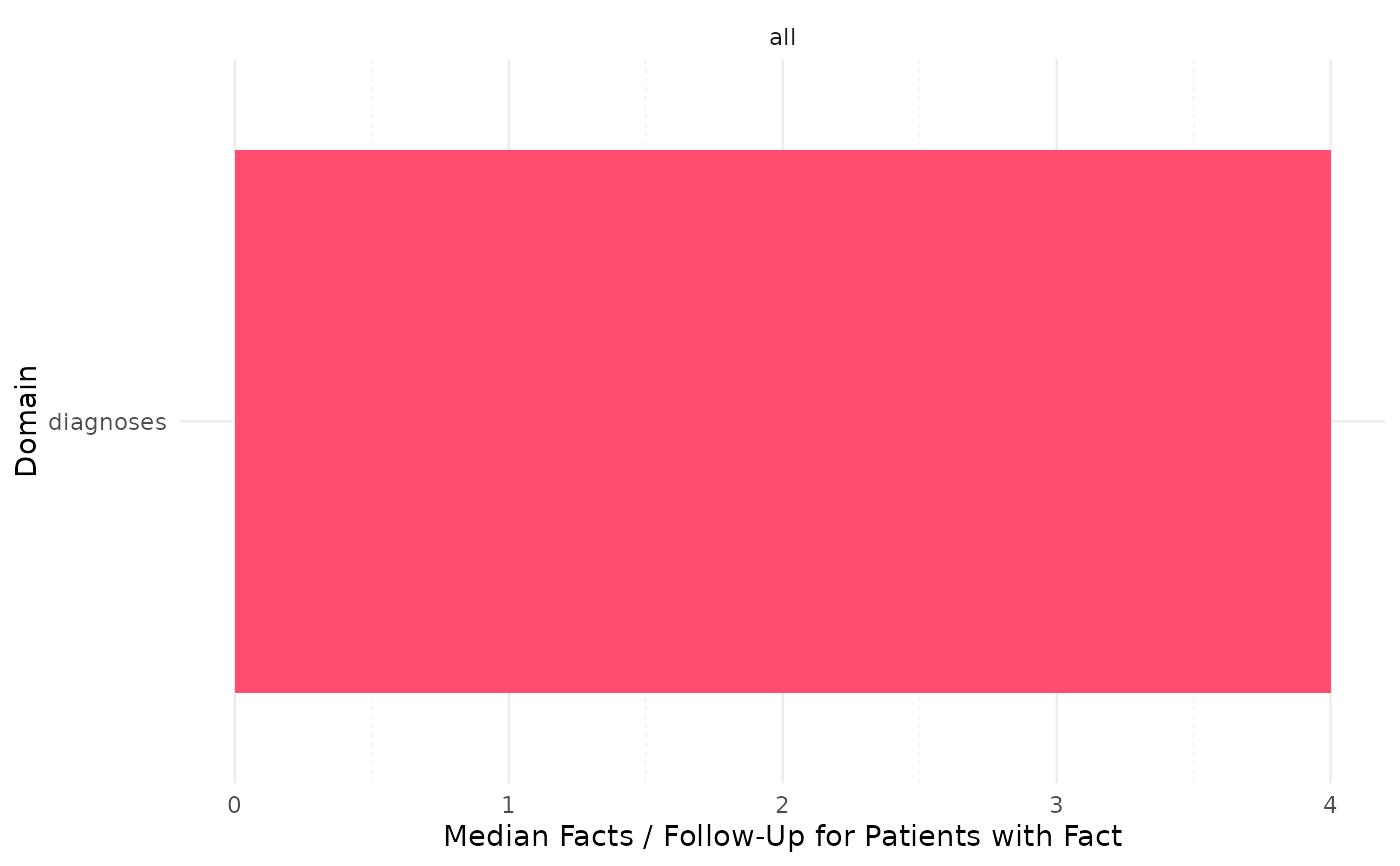
#' Execute `pf_output` function
#' The output was edited for a better indication of what the visualization will
#' look like.
#' The 0s are a limitation of the small sample data set used for this example
pf_output_example <- pf_output(process_output = pf_process_example %>%
dplyr::mutate(median_site_without0s = 4),
## tweak synthetic output for example
output = 'median_site_without0s')
pf_output_example
 #' Easily convert the graph into an interactive ggiraph or plotly object with
#' `make_interactive_squba()`
make_interactive_squba(pf_output_example)
#' Easily convert the graph into an interactive ggiraph or plotly object with
#' `make_interactive_squba()`
make_interactive_squba(pf_output_example)