Patient Facts — pf_process • patientfacts

This is a completeness module that will compute the number of facts per years of follow-up for each patient in a cohort. The user will provide the domains (domain_tbl) and visit types (visit_type_tbl) of interest. Sample versions of these inputs are included as data in the package and are accessible with patientfacts::. Results can optionally be stratified by site, age group, visit type, and/or time. This function is compatible with both the OMOP and the PCORnet CDMs based on the user's selection.

Usage

pf_process(
  cohort = cohort,
  study_name = "my_study",
  omop_or_pcornet = "omop",
  multi_or_single_site = "single",
  anomaly_or_exploratory = "exploratory",
  time = FALSE,
  time_span = c("2012-01-01", "2020-01-01"),
  time_period = "year",
  p_value = 0.9,
  age_groups = NULL,
  patient_level_tbl = FALSE,
  visit_types = c("outpatient", "inpatient"),
  domain_tbl = patientfacts::pf_domain_file,
  visit_tbl = cdm_tbl("visit_occurrence"),
  visit_type_table = patientfacts::pf_visit_file_omop
)

Arguments

cohort

tabular input || required

The cohort to be used for data quality testing. This table should contain, at minimum:

site | character | the name(s) of institutions included in your cohort
person_id / patid | integer / character | the patient identifier
start_date | date | the start of the cohort period
end_date | date | the end of the cohort period

Note that the start and end dates included in this table will be used to limit the search window for the analyses in this module.

study_name

string || defaults to my_study

A string identifier for the name of your study

omop_or_pcornet

string || required

A string, either omop or pcornet, indicating the CDM format of the data

omop: run the pf_process_omop() function against an OMOP CDM instance
pcornet: run the pf_process_pcornet() function against a PCORnet CDM instance

multi_or_single_site

string || defaults to single

A string, either single or multi, indicating whether a single-site or multi-site analysis should be executed

anomaly_or_exploratory

string || defaults to exploratory

A string, either anomaly or exploratory, indicating what type of results should be produced.

Exploratory analyses give a high level summary of the data to examine the fact representation within the cohort. Anomaly detection analyses are specialized to identify outliers within the cohort.

time

boolean || defaults to FALSE

A boolean to indicate whether to execute a longitudinal analysis

time_span

vector - length 2 || defaults to c('2012-01-01', '2020-01-01')

A vector indicating the lower and upper bounds of the time series for longitudinal analyses

time_period

string || defaults to year

A string indicating the distance between dates within the specified time_span. Defaults to year, but other time periods such as month or week are also acceptable

p_value

numeric || defaults to 0.9

The p value to be used as a threshold in the Multi-Site, Anomaly Detection, Cross-Sectional analysis

age_groups

tabular input || defaults to NULL

If you would like to stratify the results by age group, create a table or CSV file with the following columns and use it as input to this parameter:

min_age | integer | the minimum age for the group (i.e. 10)
max_age | integer | the maximum age for the group (i.e. 20)
group | character | a string label for the group (i.e. 10-20, Young Adult, etc.)

If you would not like to stratify by age group, leave as NULL

patient_level_tbl

boolean || defaults to FALSE

A boolean indicating whether an additional table with patient level results should be output.

If TRUE, the output of this function will be a list containing both the summary and patient level output. Otherwise, this function will just output the summary dataframe

visit_types

string or vector || defaults to c('outpatient', 'inpatient')

A string or vector of visit types by which the output should be stratified. Each visit type listed in this parameter should match an associated visit type defined in the visit_type_table

domain_tbl

tabular input || required

A table that defines the fact domains to be investigated in the analysis. This input should contain:

domain | character | a string label for the domain being examined (i.e. prescription drugs)
domain_tbl | character | the CDM table where information for this domain can be found (i.e. drug_exposure)
filter_logic | character | logic to be applied to the domain_tbl in order to achieve the definition of interest; should be written as if you were applying it in a dplyr::filter command in R

visit_tbl

tabular input || defaults to cdm_tbl('visit_occurrence')

The CDM table with visit information (i.e. visit_occurrence or encounter)

visit_type_table

tabular input || required

A table that defines visit types of interest called in visit_types. This input should contain:

visit_concept_id / visit_detail_concept_id or enc_type | integer or character | the visit_(detail)_concept_id or enc_type that represents the visit type of interest (i.e. 9201 or IP)
visit_type | character | the string label to describe the visit type

Value

This function will return a dataframe summarizing the distribution of facts per visit type for each user defined variable. It can also optionally return un-summarized patient-level distributions. For a more detailed description of output specific to each check type, see the PEDSpace metadata repository

Examples


#' Source setup file
source(system.file('setup.R', package = 'patientfacts'))

#' Create in-memory RSQLite database using data in extdata directory
conn <- mk_testdb_omop()

#' Establish connection to database and generate internal configurations
initialize_dq_session(session_name = 'pf_process_test',
                      working_directory = my_directory,
                      db_conn = conn,
                      is_json = FALSE,
                      file_subdirectory = my_file_folder,
                      cdm_schema = NA)
#> Connected to: :memory:@NA

## turn of SQL trace for example
config('db_trace', FALSE)

#' Build mock study cohort
cohort <- cdm_tbl('person') %>% dplyr::distinct(person_id) %>%
  dplyr::mutate(start_date = as.Date(-5000), # RSQLite does not store date objects,
                                      # hence the numerics
                end_date = as.Date(15000),
                site = ifelse(person_id %in% c(1:6), 'synth1', 'synth2'))

#' Execute `pf_process` function
#' This example will use the single site, exploratory, cross sectional
#' configuration
pf_process_example <- pf_process(cohort = cohort,
                                 study_name = 'example_study',
                                 multi_or_single_site = 'single',
                                 anomaly_or_exploratory = 'exploratory',
                                 visit_type_table =
                                   patientfacts::pf_visit_file_omop,
                                 omop_or_pcornet = 'omop',
                                 visit_types = c('all'),
                                 domain_tbl = patientfacts::pf_domain_file %>%
                                   dplyr::filter(domain == 'diagnoses')) %>%
  suppressMessages()
#> ┌ Output Function Details ─────────────────────────────────────┐
#> │ You can optionally use this dataframe in the accompanying    │
#> │ `pf_output` function. Here are the parameters you will need: │
#> │                                                              │
#> │ Always Required: process_output                              │
#> │ Required for Check: output                                   │
#> │                                                              │
#> │ See ?pf_output for more details.                             │
#> └──────────────────────────────────────────────────────────────┘

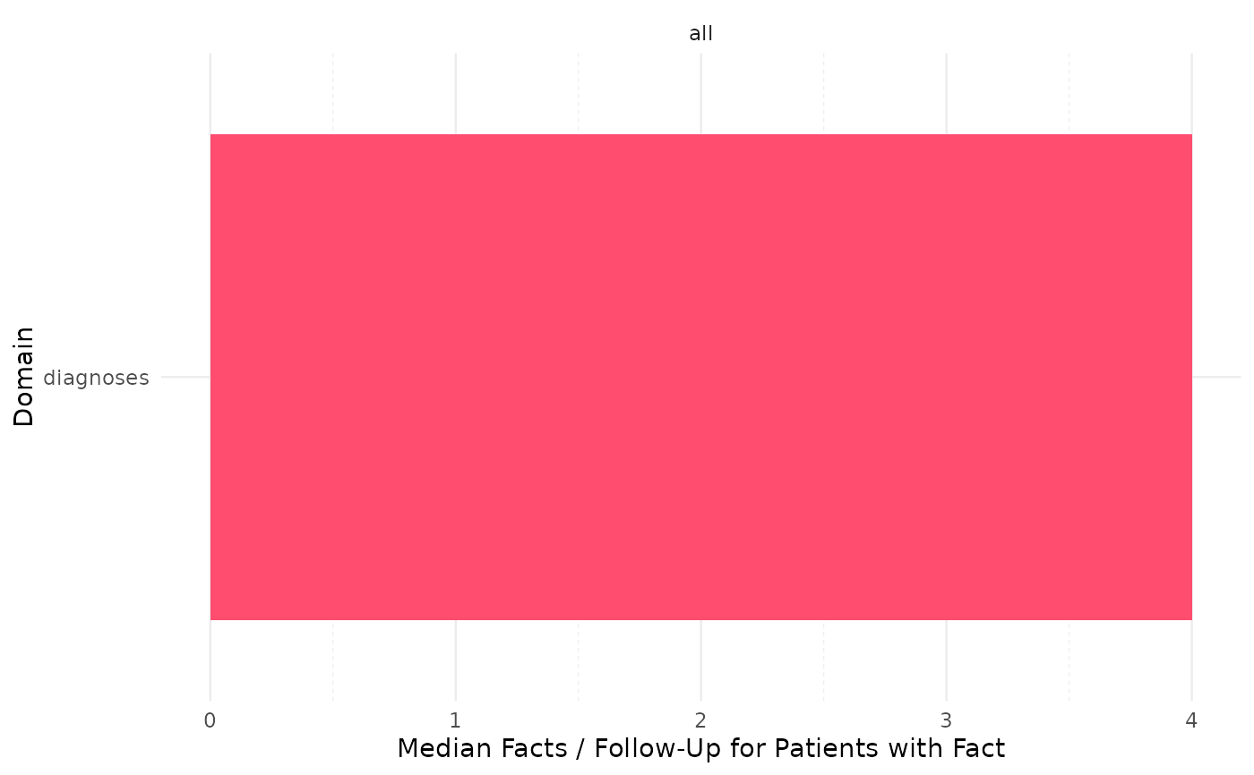
pf_process_example
#> # A tibble: 1 × 11
#>   study     site  visit_type domain median_all_with0s median_all_without0s n_tot
#>   <chr>     <chr> <chr>      <chr>              <dbl>                <dbl> <dbl>
#> 1 example_… comb… all        diagn…                 0                    0    12
#> # ℹ 4 more variables: n_w_fact <dbl>, median_site_with0s <dbl>,
#> #   median_site_without0s <dbl>, output_function <chr>

#' Execute `pf_output` function
#' The output was edited for a better indication of what the visualization will
#' look like.
#' The 0s are a limitation of the small sample data set used for this example
pf_output_example <- pf_output(process_output = pf_process_example %>%
                                 dplyr::mutate(median_site_without0s = 4),
                                 ## tweak synthetic output for example
                               output = 'median_site_without0s')

pf_output_example


#' Easily convert the graph into an interactive ggiraph or plotly object with
#' `make_interactive_squba()`

make_interactive_squba(pf_output_example)