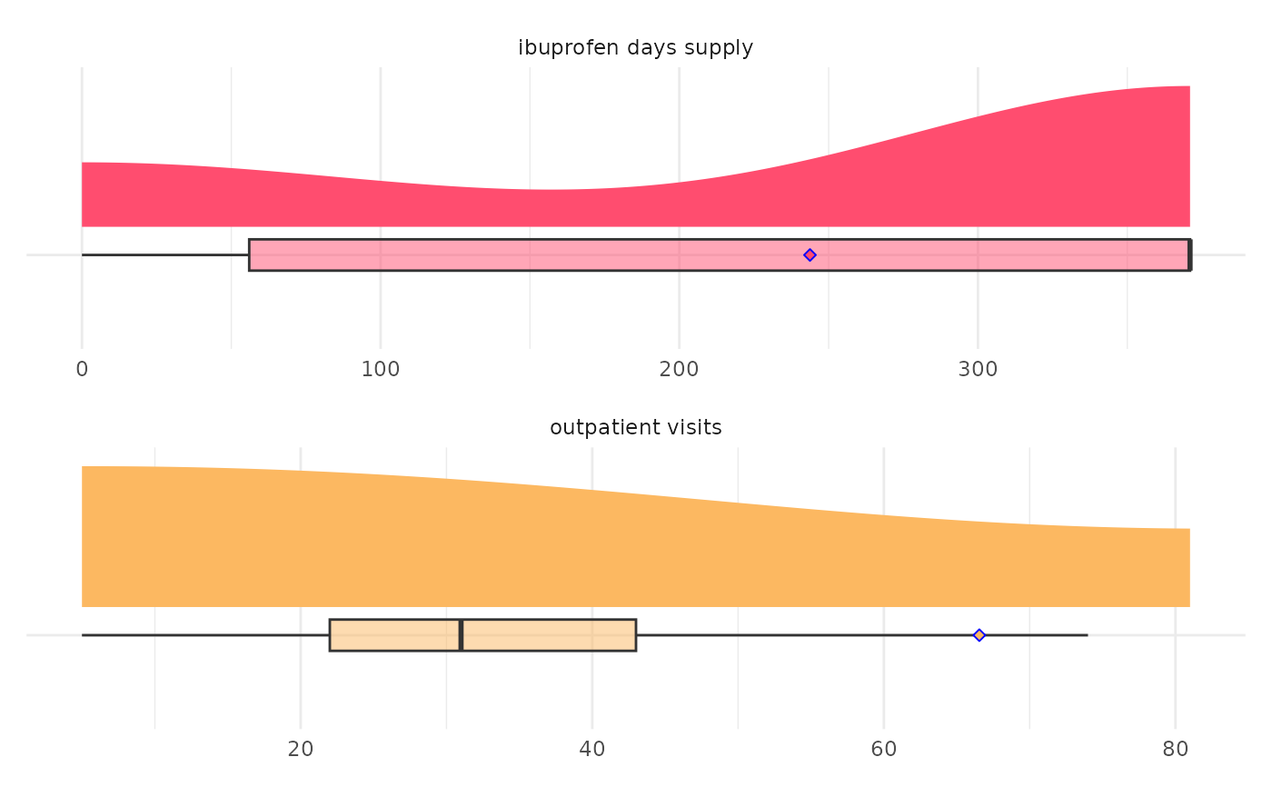
Using the tabular output generated by qvd_process, this function will build a graph to
visualize the results. Each function configuration will output a bespoke ggplot. Theming can
be adjusted by the user after the graph has been output using + theme(). Most graphs can
also be made interactive using make_interactive_squba()
Usage
qvd_output(
  process_output,
  value_type_filter = NULL,
  frequency_min = 5,
  display_outliers = FALSE,
  summary_stat = "mean",
  large_n = FALSE,
  large_n_sites = NULL
)
Arguments
- process_output
tabular input || required
The tabular output produced by
qvd_process- value_type_filter
string or vector || defaults to
NULLA string or vector of strings to filter the graph to specific variables of interest.
A single variable is required to be input in this parameter for the
Multi-Site, Anomaly Detection, Longitudinalcheck. For all others, it is not required but we recommend limiting to 5 variable or fewer to maintain visibility.- frequency_min
integer || defaults to
5An integer indicating the minimum amount of times a value should occur to be included in the output. This parameter is aimed at trimming infrequently occurring outliers for a cleaner plot.
- display_outliers
boolean || defaults to
FALSEFor boxplot output, a boolean to indicate whether outliers should be displayed
- summary_stat
string || defaults to
meanA string indicating the summary statistic that should be displayed on the plot. This is a required for each
Exploratory, Longitudinaloutput.Acceptable values are
mean,median,q1,q3, orsd- large_n
boolean || defaults to
FALSEFor Multi-Site analyses, a boolean indicating whether the large N visualization, intended for a high volume of sites, should be used. This visualization will produce high level summaries across all sites, with an option to add specific site comparators via the
large_n_sitesparameter.- large_n_sites
vector || defaults to
NULLWhen
large_n = TRUE, a vector of site names that can add site-level information to the plot for comparison across the high level summary information.
Value
This function will produce a graph to visualize the results
from qvd_process based on the parameters provided. The default
output is typically a static ggplot or gt object, but interactive
elements can be activated by passing the plot through make_interactive_squba.
For a more detailed description of output specific to each check type,
see the PEDSpace metadata repository
Examples
#' Source setup file
source(system.file('setup.R', package = 'quantvariabledistribution'))
#' Create in-memory RSQLite database using data in extdata directory
conn <- mk_testdb_omop()
#' Establish connection to database and generate internal configurations
initialize_dq_session(session_name = 'qvd_process_test',
working_directory = my_directory,
db_conn = conn,
is_json = FALSE,
file_subdirectory = my_file_folder,
cdm_schema = NA)
#> Connected to: :memory:@NA
#' Build mock study cohort
cohort <- cdm_tbl('person') %>% dplyr::distinct(person_id) %>%
dplyr::mutate(start_date = -10000, # RSQLite does not store date objects,
# hence the numerics
end_date = 30000,
site = ifelse(person_id %in% 1:6, 'synth1', 'synth2'))
#' Create `qvd_value_file` input
qvd_input <- dplyr::tibble('value_name' = c('ibuprofen days supply',
'outpatient visits'),
'domain_tbl' = c("drug_exposure",
'visit_occurrence'),
'value_field' = c('days_supply',
'person_id'),
'date_field' = c('drug_exposure_start_date',
'visit_start_date'),
'concept_field' = c('drug_concept_id',
NA),
'codeset_name' = c('rx_ibuprofen',
NA),
'filter_logic' = c(NA,
'visit_concept_id == 9202'))
#' Execute `qvd_process` function
#' This example will use the single site, exploratory, cross sectional
#' configuration
qvd_process_example <- qvd_process(cohort = cohort,
multi_or_single_site = 'single',
anomaly_or_exploratory = 'exploratory',
time = FALSE,
omop_or_pcornet = 'omop',
qvd_value_file = qvd_input) %>%
suppressMessages()
#> ┌ Output Function Details ──────────────────────────────────────┐
#> │ You can optionally use this dataframe in the accompanying │
#> │ `qvd_output` function. Here are the parameters you will need: │
#> │ │
#> │ Always Required: process_output │
#> │ Optional: display_outliers, frequency_min, value_type_filter │
#> │ │
#> │ See ?qvd_output for more details. │
#> └───────────────────────────────────────────────────────────────┘
qvd_process_example
#> # A tibble: 261 × 10
#> site value_col value_freq value_type mean_val median_val sd_val q1_val
#> <chr> <int> <int> <chr> <dbl> <dbl> <dbl> <dbl>
#> 1 combined 0 47 ibuprofen da… 244. 371 156. 56
#> 2 combined 1 2 ibuprofen da… 244. 371 156. 56
#> 3 combined 2 2 ibuprofen da… 244. 371 156. 56
#> 4 combined 3 1 ibuprofen da… 244. 371 156. 56
#> 5 combined 7 30 ibuprofen da… 244. 371 156. 56
#> 6 combined 11 1 ibuprofen da… 244. 371 156. 56
#> 7 combined 14 3 ibuprofen da… 244. 371 156. 56
#> 8 combined 18 1 ibuprofen da… 244. 371 156. 56
#> 9 combined 19 7 ibuprofen da… 244. 371 156. 56
#> 10 combined 21 4 ibuprofen da… 244. 371 156. 56
#> # ℹ 251 more rows
#> # ℹ 2 more variables: q3_val <dbl>, output_function <chr>
#' Execute qvd_output` function
qvd_output_example <- qvd_output(process_output = qvd_process_example)
qvd_output_example
 #' Easily convert the graph into an interactive ggiraph or plotly object with
#' `make_interactive_squba()`
make_interactive_squba(qvd_output_example)
#' Easily convert the graph into an interactive ggiraph or plotly object with
#' `make_interactive_squba()`
make_interactive_squba(qvd_output_example)