This is a plausibility module that will evaluate the distribution of either quantitative
variables (i.e. drug dosages) or the distribution of patient counts (i.e. patients with
inpatient visits). The user will provide definitions for the variables to be
examined (qvd_value_file). Sample versions of this input are included as
data in the package and are accessible with quantvariabledistribution::.
Results can optionally be stratified by site, age group, and/or time. This
function is compatible with both the OMOP and the PCORnet CDMs based on the user's
selection.
Usage
qvd_process(
  cohort,
  qvd_value_file,
  multi_or_single_site = "single",
  anomaly_or_exploratory = "exploratory",
  omop_or_pcornet,
  time = FALSE,
  time_span = c("2012-01-01", "2020-01-01"),
  time_period = "year",
  age_groups = NULL,
  sd_threshold = 2,
  kl_log_base = "log2",
  euclidean_stat = "mean"
)
Arguments
- cohort
tabular input || required
The cohort to be used for data quality testing. This table should contain, at minimum:
site| character | the name(s) of institutions included in your cohortperson_id/patid| integer / character | the patient identifierstart_date| date | the start of the cohort periodend_date| date | the end of the cohort period
Note that the start and end dates included in this table will be used to limit the search window for the analyses in this module.
- qvd_value_file
tabular input || required
A dataframe or CSV file with information about each of the variables that should be examined in the function. Should contain the following columns:
value_name| string | a string label for the value variabledomain_tbl| character | CDM table where the value data is foundvalue_field| character | the name of the field with the quantitative variable OR the name of the person identifier column for patient count checksdate_field| character | a date field in thedomain_tblthat should be used for temporal filteringconcept_field| character | the string name of the field in the domain table where the concepts are located (only needed when codeset is provided)codeset_name| character | optional field to include the name of a codeset filevocabulary_field| character | for PCORnet applications, the name of the field in the domain table with a vocabulary identifier to differentiate concepts from one another (ex: dx_type); can be set to NA for OMOP applicationsfilter_logic| character | logic to be applied to the domain_tbl in order to achieve the definition of interest; should be written as if you were applying it in a dplyr::filter command in R
To see an example of what this input should look like, see
?quantvariabledistribution::qvd_value_file_omopor?quantvariabledistribution::qvd_value_file_pcornet- multi_or_single_site
string || defaults to
singleA string, either
singleormulti, indicating whether a single-site or multi-site analysis should be executed- anomaly_or_exploratory
string || defaults to
exploratoryA string, either
anomalyorexploratory, indicating what type of results should be produced.Exploratory analyses give a high level summary of the data to examine the fact representation within the cohort. Anomaly detection analyses are specialized to identify outliers within the cohort.
- omop_or_pcornet
string || required
A string, either
omoporpcornet, indicating the CDM format of the data- time
boolean || defaults to
FALSEA boolean to indicate whether to execute a longitudinal analysis
- time_span
vector - length 2 || defaults to
c('2012-01-01', '2020-01-01')A vector indicating the lower and upper bounds of the time series for longitudinal analyses
- time_period
string || defaults to
yearA string indicating the distance between dates within the specified time_span. Defaults to
year, but other time periods such asmonthorweekare also acceptable- age_groups
tabular input || defaults to
NULLIf you would like to stratify the results by age group, create a table or CSV file with the following columns and use it as input to this parameter:
min_age| integer | the minimum age for the group (i.e. 10)max_age| integer | the maximum age for the group (i.e. 20)group| character | a string label for the group (i.e. 10-20, Young Adult, etc.)
If you would not like to stratify by age group, leave as
NULL- sd_threshold
integer || defaults to
2An integer indicating the number of standard deviations a value should fall away from the mean to be considered an outlier. This will be applied to each of the
Single Site, Anomaly Detectionchecks- kl_log_base
string || defaults to
log2A string indicating the log base that should be used for the Kullback-Liebler divergence computation
Acceptable values are:
log,log2,log10- euclidean_stat
string || defaults to
meanA string indicating the summary statistic that should be used for the euclidean distance computation in the
Multi-Site, Anomaly Detection, LongitudinalcheckAcceptable values are
meanormedian
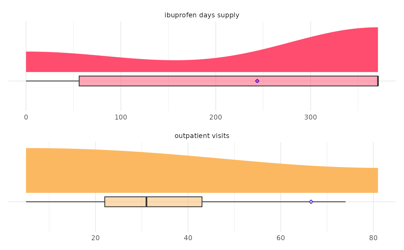
Value
This function will return a dataframe summarizing the frequency distribution of each quantitative variable. For a more detailed description of output specific to each check type, see the PEDSpace metadata repository
Examples
#' Source setup file
source(system.file('setup.R', package = 'quantvariabledistribution'))
#' Create in-memory RSQLite database using data in extdata directory
conn <- mk_testdb_omop()
#' Establish connection to database and generate internal configurations
initialize_dq_session(session_name = 'qvd_process_test',
working_directory = my_directory,
db_conn = conn,
is_json = FALSE,
file_subdirectory = my_file_folder,
cdm_schema = NA)
#> Connected to: :memory:@NA
#' Build mock study cohort
cohort <- cdm_tbl('person') %>% dplyr::distinct(person_id) %>%
dplyr::mutate(start_date = -10000, # RSQLite does not store date objects,
# hence the numerics
end_date = 30000,
site = ifelse(person_id %in% 1:6, 'synth1', 'synth2'))
#' Create `qvd_value_file` input
qvd_input <- dplyr::tibble('value_name' = c('ibuprofen days supply',
'outpatient visits'),
'domain_tbl' = c("drug_exposure",
'visit_occurrence'),
'value_field' = c('days_supply',
'person_id'),
'date_field' = c('drug_exposure_start_date',
'visit_start_date'),
'concept_field' = c('drug_concept_id',
NA),
'codeset_name' = c('rx_ibuprofen',
NA),
'filter_logic' = c(NA,
'visit_concept_id == 9202'))
#' Execute `qvd_process` function
#' This example will use the single site, exploratory, cross sectional
#' configuration
qvd_process_example <- qvd_process(cohort = cohort,
multi_or_single_site = 'single',
anomaly_or_exploratory = 'exploratory',
time = FALSE,
omop_or_pcornet = 'omop',
qvd_value_file = qvd_input) %>%
suppressMessages()
#> ┌ Output Function Details ──────────────────────────────────────┐
#> │ You can optionally use this dataframe in the accompanying │
#> │ `qvd_output` function. Here are the parameters you will need: │
#> │ │
#> │ Always Required: process_output │
#> │ Optional: display_outliers, frequency_min, value_type_filter │
#> │ │
#> │ See ?qvd_output for more details. │
#> └───────────────────────────────────────────────────────────────┘
qvd_process_example
#> # A tibble: 261 × 10
#> site value_col value_freq value_type mean_val median_val sd_val q1_val
#> <chr> <int> <int> <chr> <dbl> <dbl> <dbl> <dbl>
#> 1 combined 0 47 ibuprofen da… 244. 371 156. 56
#> 2 combined 1 2 ibuprofen da… 244. 371 156. 56
#> 3 combined 2 2 ibuprofen da… 244. 371 156. 56
#> 4 combined 3 1 ibuprofen da… 244. 371 156. 56
#> 5 combined 7 30 ibuprofen da… 244. 371 156. 56
#> 6 combined 11 1 ibuprofen da… 244. 371 156. 56
#> 7 combined 14 3 ibuprofen da… 244. 371 156. 56
#> 8 combined 18 1 ibuprofen da… 244. 371 156. 56
#> 9 combined 19 7 ibuprofen da… 244. 371 156. 56
#> 10 combined 21 4 ibuprofen da… 244. 371 156. 56
#> # ℹ 251 more rows
#> # ℹ 2 more variables: q3_val <dbl>, output_function <chr>
#' Execute qvd_output` function
qvd_output_example <- qvd_output(process_output = qvd_process_example)
qvd_output_example
 #' Easily convert the graph into an interactive ggiraph or plotly object with
#' `make_interactive_squba()`
make_interactive_squba(qvd_output_example)
#' Easily convert the graph into an interactive ggiraph or plotly object with
#' `make_interactive_squba()`
make_interactive_squba(qvd_output_example)